A Daubert Challenge to the Pearson Correlation Coefficient
Author
AE Rodriguez
Published
December 3, 2025
Attorneys in litigation proceedings will sometimes file a legal motion known as a Daubert challenge against opposing party’s economics expert. The objective of the motion is is to exclude the expert’s testimony. The claim questions not the expert’s conclusion; rather, the intention is to impeach the experts methodology, alleging it is not reliable, applicable, or relevant.
The motion compels the judge, acting as a “gatekeeper” scrutinizing expert evidence, to appraise the approach being used by the expert. The challenge focuses on the methodology’s scientific validity by evaluating factors like testability, peer review, error rates, and general acceptance within the relevant field.
In a recent contracts termination matter where we were experts for plaintiff - who suffered losses as a consequence of the incident - we used a well-known, conventional approach to calculating lost profits: a method known as the “yardstick method.”
The yardstick method is one of two popular approaches to envisioning and determining what would have happened to plaintiffs but for the incident; put differently, what would the counterfactual or but-for world have looked like?
Alternatively to the yardstick approach is the, before-and-after method. The before-and-after method projects a firm’s own past performance into the future.
This is opposing counsel’s argument on the Daubert Challenge.
D. The Experts’ “Correlation Coefficient” Exercise Is Misleading and Has No Basis in the Facts or the Data
In their Report, the Experts attempt to validate their “CTIS Index” model by calculating a statistical correlation between DEFENDANTS’s projected “but-for” income—derived from their self-constructed index—and PLAINTIFF’s total revenues from 2016 to 2023. Based on their resulting correlation coefficient of 0.97, the Experts assert that “the CTIS Index is representative of the market in which DEFENDANT and PLAINTIFF participate.
Its most likely that opposing counsel got their wanties in a pad because we did not use the typical linear regression model typically applied. The “yardstick” we created was a volume-weighted composite index of plaintiff’s competitors based on plaintiff’s disclosed NAICS categories. To demonstrate it was truly representative and therefore suitable we argued that the high (Pearson) correlation coefficient between the yardstick and plaintiff’s historical sales performance was probative. Moreover, multiple linear regression is far more complex than the simple algebra underlying a volume-weighted index of competitors.
This is what triggered the challenge. True story. I’m not sure whether opposing counsel could have picked something that would be more of a turkey than challenging and algebraic index and the use of the Pearson correlation coefficient to measure association between two series; reeks of desperation.
The pearson correlation appraises the relationship between two variables, two series, based on the similarity of their trend and direction. Pearson’s primacy over the thousands of available measures of association is its simplicity and interpretability; it returns the magnitude and direction of the association between two variables. Moreover, critical value tables, which are needed to determine the statistical significance of the resulting correlation are readily available.
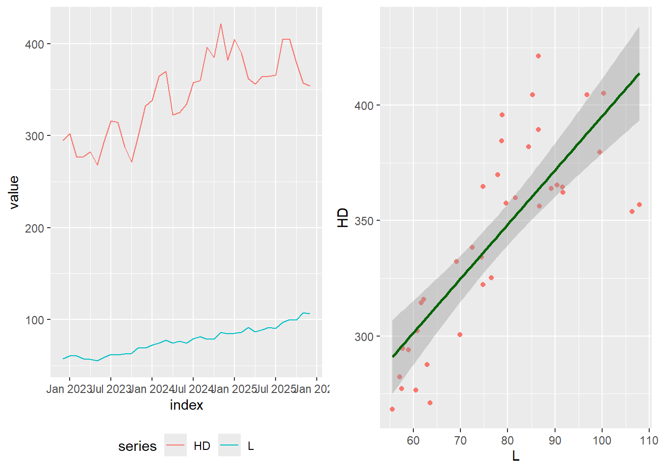
Importantly, it is unlikely that an alternative measure of association like Spearmans Correlation would return a contrary finding. Lets take a look at a simulation of two NAICS related series. Loews and Home Depot are competitors both reporting under the same NAICS code. We test to see if there is no correlation between them. Put differently, whether these two firms are “related.” “Related” to be answered in the affirmative if the test of no correlation is rejected. The test is rejected if the p-value is smaller than 0.05.
We test Pearson and Spearmans Correlation coefficients.
suppressWarnings({suppressPackageStartupMessages({library(tidyverse)library(dtw)library(TSclust)library(TSstudio)library(arsenal)library(quantmod)library(knitr)})})# Download two series from Yahoo Finance# Home Depot & Loewssymbols <-c("L", "HD")getSymbols(symbols, from =Sys.Date() -years(3), src ="yahoo")
As noted above in the extract from our Report cited by opposing counsel: we chose the set of firms for the Yardstick Index from companies reporting within the same 6-digit NAICS codes. The NAICS code is our grouping variable; in fact “the beauty of this is its simplicity” - well put by Walter and the Dude.
What if, instead - like the Dude: “you are not into the whole brevity thing?You could go big. You could use Pearson Correletion as the grouping variable; and for good measure also take a look at a comparator known as Dynamic Time Warping or DTW. In its similarity calculation DTW accounts for the variation in the speed or time (unsynchronized) of the time series examined.
Here we propose to use the Pearson Correlation and DTW to appraise whether they are suitable to identify whether companies are “related.” Formally, we cluster different groups.
Ill pick AAPL, MSFT, GOOGL, AMZN, JPM, GS, L, and HD. All use multiple codes given that they are all large diversified operations operating multiple lines of business.
AAPL (Apple): Codes include 334220 (Radio and Television Broadcasting and Wireless Communications Equipment Manufacturing), 334111 (Electronic Computer Manufacturing), and retail codes like 443143 (Appliance, Television and Other Electronics Stores).
MSFT (Microsoft):513210 (Software Publishers).
GOOGL (Alphabet/Google):519130 (Internet Publishing and Broadcasting and Web Search Portals).
AMZN (Amazon):454110 (Electronic Shopping and Mail-Order Houses).
hc_cor <-hclust(cor_dist_mat, method ="ward.D") hc_dtw <-hclust(dtw_dist_mat, method ="ward.D") # Plot the dendrogram to visualize the clusters#plot(hc_cor, main = "Hierarchical Clusterings", # xlab = "Prices", ylab = "Distance")#plot(hc_dtw, main = "Hierarchical Clusterings", # xlab = "Prices", ylab = "Distance")k_clusters =3clusters_cor =cutree(hc_cor, k = k_clusters)clusters_dtw =cutree(hc_dtw, k = k_clusters)#print(clusters)myclusters =cbind(clusters_cor, clusters_dtw)knitr::kable(myclusters, caption ="Grouping Results",col.names =c("Pearson", "DTW"),align =c("c", "c") )
Grouping Results
Pearson
DTW
AAPL
1
1
MSFT
2
2
GOOGL
1
1
AMZN
2
1
JPM
2
1
GS
2
2
L
2
3
HD
3
2
Clearly, it is possible to assemble the comparison group using clustering methods. Interpretable yes; but its not simple because of the many possible permutations encompassing distance metrics chose, clustering methods, number of clusters selected. It would be a pinata for any cross-examination.
Write to me:
A.E. Rodriguez, PhD Professor Economics & Business Analytics Pompea College of Business University of New Haven